
TPS Optimization Algorithms
Treatment planning involves a balancing act between competing clinical goals. For example, a target (tumor) should ideally receive a full prescription dose while the surrounding healthy organs should receive as close to zero dose as is achievable. The goal of plan optimization, then, is to find an optimal trade-off between inherently conflicting clinical goals given the set of treatment delivery limitations.
Optimization Parameters
Cost function
Cost functions, also known as objective functions, quantify the degree to which a treatment plan meets its competing objectives. The goal of all optimizers is to minimize the cost function by modifying the dose distribution within the constraints of clinical deliverability.

Dose-Volume Histogram (DVH) Constraints
- dmax refers to the maximum dose.
- dmin refers to the minimum dose.
- Volume at dose: V(x)[dose unit] [<, >, =] y[volume unit]
- Constrains the volume of a structure receiving a given dose.
- Example: V20Gy<30% indicates that the volume receiving 20Gy should be less than 30% of the structure’s total volume.
- x[Dose unit] indicates the amount of dose to quantify volume against. Units typically Gy or % of prescription dose.
- [<, >, =] indicates the direction of the constraint.
- y[volume unit] indicates the volume being constrained at the given dose level. Units typically cc or % of structure volume.
- Dose at volume: D(y)[volume unit] [<, >, =] (x)[dose unit]
- Constrains the dose that a given volume of a structure may receive.
- Example: D95% >50.4Gy indicates that 95% of the structure’s total volume should receive more than 50.4Gy.

Equivalent Uniform Dose (EUD) Constraints
Equivalent Uniform Dose (EUD) is defined as the dose that, if homogeneously delivered to an anatomical structure, causes the same expected number of cells to survive as the actual non-homogeneous dose distribution does. Equivalent Uniform Dose allows a user to directly constrain the dose distribution according to a specified dose, d, and the degree to which the organ in is serial or parallel, α.
What should α value to use
- Parallel organs should be given an α of 1.
- Note that in this case, EUD reduced to mean dose.
- Serial organs may be given an α of 10.
- This approximates a maximum dose constraint.
- Targets may also be constrained with EUD by using negative values of α.
Common Optimization Algorithms
| Fluence Map Optimization (FMO) | Direct Machine Parameter Optimization (DMPO) | Multi-Criteria (Pareto) Optimization (MCO) | |
|---|---|---|---|
| Overview | Optimizes the fluence map then attempts to achieve this fluence pattern using real machine parameters. | The optimizer directly acts on segment parameters such as MLC leaf position and segment weight to yield the best achievable dose distribution. | The optimizer generates a series of Pareto optimal plans and allows the user to choose between them. Pareto optimal plans are those plan where a given parameter cannot be improved without hurting another parameter. |
| Advantages |
|
|
|
| Disadvantages |
|
|
|
Fluence Map Optimization (FMO)
Fluence Map Optimization (FMO) uses gradient based methods (1st and 2nd derivatives) to arrive at an optimal fluence distribution. Once the optimal fluence distribution is found, leaf-sequencing is used to find a set of machine deliverable apertures which approximate this ideal fluence map. Note, the actual deliverable fluence map will not match the ideally calculated fluence map due to machine limitations.
Advantages of FMO
- FMO is computationally inexpensive (fast) compared to Direct Aperture Optimization.
- A global optimum fluence map can always be found because the cost function with associated delivery constraints is convex.
- I.e. For convex functions, a local minimizer is a global minimizer.
Disadvantages of FMO
- Because machine parameters are not directly optimized, the final dose distribution after leaf-sequencing is unlikely to represent the best possible dose distribution the machine could produce.
Direct Machine Parameter Optimization (DMPO)
Direct Machine Parameter Optimization (DMPO), sometimes referred to as Direct Aperture Optimization, is a plan optimization method that directly considers leaf position and segment weights as variables during optimization. VMAT implementations of DMPO also consider other machine parameters such as gantry, couch, and collimator limitations. DMPO produces a plan that has been optimized with actual machine parameters in mind yielding a more optimal final dose distribution than FMO.
The additional machine limitations constrain the possible optimizer solutions resulting in an optimization problem that is nonlinear and nonconvex. This means that there are locally optimal solutions which are not globally optimal. As a result, gradient methods like those used in FMO are less likely to find the absolute best solution. Put another way; the optimizer can get "stuck" in a poor solution because all small variations on the machine parameters yield a worse plan even when large changes to the machine parameters might yield a very good plan.
Approaches to solving nonconvex optimization problems
Simulated Annealing
- Periodically introduces random changes to the variables. The optimizer evaluates the random changes and only retains those which improve the cost function.
- This allows the optimizer to escape from local minima in nonconvex problems.
- The idea of simulated annealing is taken from metallurgy where annealing, by periodically adding heat (randomness), allows the metal to cool into harder (lower energy) states.
Column generation methods
- Divides the optimization problem into subproblems, such as an individual aperture position, and attempts to optimize them. The optimizer then works on the global problem by optimizing segment weights.
Gradient-based methods
- Uses the derivative and second derivative of a problem to determine the direction of optimization.
Genetic methods
- Creates a population of possible solutions and uses “survival of the fittest” to create increasingly optimal solutions.
Multi-Criteria Optimization (MCO)
Traditional plan optimization – FMO and DMPO – assigns manual weights DVH objectives in an attempt to yield the optimal plan. These DVH objectives and weights are, unfortunately, often not directly associated with the desired clinical goal. This means that traditional optimization is a time consuming trial-and-error process. Multi-criteria optimization attempts to resolve these issues by tying clinical desires more directly to optimization.
Prioritized Optimization
- Clinical objectives are determined and ranked in the optimizer.
- Example rankings
- Spinal Cord: Dmax < 45Gy
- PTV: D95% = 70Gy
- Larynx: V50Gy < 27%
- Example rankings
- The optimizer attempts to achieve the ranked clinical goals in such a way that no lower ranked objective is met at the expense of a higher ranked priority.
- This is a good solution assuming that the user knows in advance what trade-offs he/she is willing to make.
- Prioritized optimization’s weakness is that it will ignore even large benefits to a lower ranked objective even if the cost to a higher ranked objective is minimal and the trade-off may be desirable.
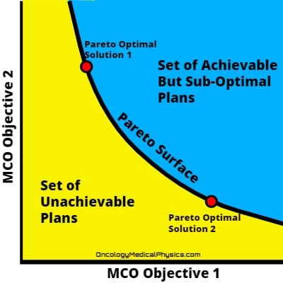
Pareto-Optimality
A plan is Pareto-optimal when it is not possible to improve the plan with respect to one objective without worsening it with respect to another objective. That is, when the plan is as good as it can be without making a trade-off.
Pareto-surface is the set of all Pareto-optimal plans. A Pareto-surface is generated by optimizing, usually by Direct Machine Parameter Optimization, a set of Pareto-optimal plans. These plans are then interpolated providing the set of plans along the Pareto-surface. The clinically optimal plan is assumed to fall somewhere along the Pareto-surface. Practically then, MCO resolves around producing and navigating the set of plans on the pareto-surface.
Viewing the trade-offs between Pareto-optimal plans is referred to as “navigating the Pareto surface.” The two most common ways to navigate the Pareto-surface are the library method and the graphic user interface (slider) method.
The library method presents a small sub-set of Pareto optimal plans. The user may choose a plan for delivery or select several plans with desirable characteristics. The selected plans may be interpolated along the Pareto surface to generate additional treatment options.
The graphic user interface method presents the user with trade-off sliders. This allows the user directly to explore the planning trade-offs to be made in Pareto optimal plans.
Navigation
Not a Member?
Sign up today to get access to hundreds of ABR style practice questions.