
MRI Design and Operation
Quick Reference
- Signal source results from atoms with unpaired protons.
- Primarily Hydrogen
- Also: O, F, Na, and K
- Magnetic Field Strength: 0.1T - 7T (earth's magnetic field is 6.5x10⁻⁵T)
- Increased field strength increases signal-to-noise ratio but also increases geometric distortions.
- The precession frequency is given by the Larmor equation

- Gradient coils are responsible for the loud noise an MRI makes.
- Signal strength (S) is proportional to square of the magnetic field (B).

Contrast Weighting
| Short TR (TR = T1) | Long TR (TR > T1) | |
| Long TE (TE = T2) | Not clinically useful | T2 weighted image |
| Short TE (TE < T2) | T1 weighted image | Proton density image |
- T2 is much smaller than T1 (milliseconds versus seconds).
- A reliable way to distinguish T1 and T2 weighting is to looks at fluid-filled structures which will appear dark on T1 weighted images and bright on T2 weighted images.
Theory of Operation
Basic Steps in Imaging
- A strong magnetic field (0.1T - 7T) is applied to the patient aligning hydrogen atoms (parallel and anti-parallel) with the field.
- Parallel alignment is only slightly preferred (~3ppm/T). This small fraction will generate the detectable signal for imaging!
- Once aligned, the protons precess about their poles at a frequency given by the Larmor Frequency equation.
- A resonant radio frequency (RF) pulse of Larmor Frequency is used to excite the aligned atoms.
- Excitation causes the amplitude of their precession to increase but does not impact the frequency.
- After the pulse, the excited atoms return to their lower energy state by emitting RF waves at their Larmor frequency.
- Receiving coils detect the emitted RF waves, recording their signal.
Voxel Encoding
The signal the receiving coils detects does not in itself contain any information except for the intensity and frequency of RF return. In order to use that signal to generate an image, one must be able to determine where that signal is coming from. Therefore, the signal is encoded along the three Cartesian axes as outlined below.
1. Slice Selection
The first method of encoding is to selectively excite only 1 slice at a time.
- A gradient magnetic field is applied in addition to the uniform magnetic field. This causes the Larmor frequency to vary as a function of position along the direction of the field gradient.
- Slices of variable width may be selected by changing the RF pulse frequency and bandwidth.
2. Phase Encoding
A temporary small gradient is briefly superimposed in a direction perpendicular to the slice selecting direction. This speeds the atoms on one side of the slice while slowing atoms on the other side. When this gradient is shut off, all the atoms return to their original precession frequency but they are now at different phases. At this point, both slice and row can be determined.
3. Frequency Encoding
The final step again uses gradient coils to create a magnetic field gradient along the axis perpendicular to both the slice selection axis and the phase encoding axis. This gradient is left on during readout.
Image Reconstruction
It is important to realize that, although each voxel’s location is encoded by phase and frequency, all voxels in a row are read out simultaneously. This data must be deconvolved by an Inverse Fourier Transform in K-space. K-space is an image that maps frequency rather than physical x-y coordinates. Once this is complete, the information may be used to generate an image.
For k-space maps, pixels near the center correspond to low-frequency data while pixels near the edge correspond to high frequency (edges).


Source of Tissue Contrast (T1 and T2 relaxation)
There are two sources of signal that can be imaged. First, changes to the number of protons aligned parallel and anti-parallel to the magnetic field called longitudinal magnetization. Longitudinal magnetization rate is characterized by T1 time.
T1 (Longitudinal Relaxation): This is the time it takes for the bulk magnetization to regrow to 63% of its equilibrium value. T1 relaxation is sometimes called spin-lattice relaxation because it is the time that it takes for the protons to realign with the magnetic field.
The second method is to measure the component of their magnetization that is orthogonal to the direction of the magnetic field (referred to as transverse magnetization). Normally the phases of precession are randomly distributed and the total transverse magnetization is zero. But immediately after excitation the phases become aligned and a signal can be detected. Random magnetic disturbances rapidly decay this signal in a precess called Free Induction Decay (FID). Rate of FID is characterized by the T2 time.
T2 (Transverse Relaxation): This is the time required after excitation for the transverse magnetization to decay to 37% of its maximum value.
Scan Parameters
Repetition time (TR): The time between excitation RF pulses. During this time, both T1 and T2 relaxation occur to varying degrees.
Echo time (TE): The time between excitation and signal acquisition.
Choice of TR and TE is driven by the T1 and T2 times of the tissues being distinguished. Timing is chosen to maximize the difference in signal intensity. For instance, if two tissues have very different T1 times we might use a TR time approximately equal to the shorter of the two tissues T1 time and a very short TE time. Reciprocally, if the two tissues have similar T1 times but differences in T2, we might use a long TR time to allow full recovery of longitudinal magnetization in both tissues but then choose a TE time that maximizes the difference in T2 decay.
Key Point: What is an echo?
An echo in MRI is similar to a sound echo in that it is a return of the FID signal at some time after the initial FID. The echo is generated by first using a 90-degree flip angle then, at time TE/2 employing a 180-degree flip angle. Echo imaging allows for rapid acquisition (multiple echoes) and fine control of contrast weighting.
Flip Angle: The angle by which the net magnetization is directed away from the magnetic field. Flip angle can be adjusted by changing the amount of energy transmitted by the RF pulse. Common flip angles are 90 degrees and 180 degrees. Flip angles are used to adjust contrast and to create echo time based weighting, such as Fluid Attenuation Inversion Recovery (FLAIR).
Time of Inversion (TI): Inversion recovery sequences operate by initially inverting the magnetization with a 180-degree pulse, then allowing some degree of T1 recovery prior to emitting a 90-degree pulse to yield contrast. TI is the time between this initial 180-degree pulse and the subsequent 90-degree pulse.

Key Point: TR controls the T1 weighting of the image. TE controls the T2 weighting of the image.
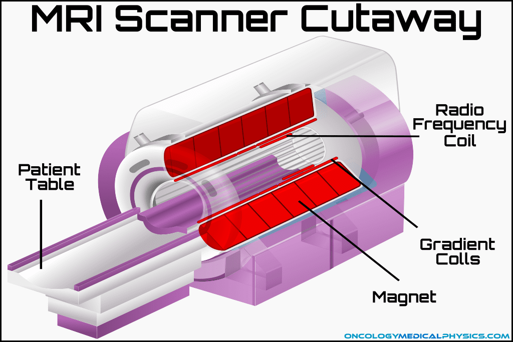
Scanner Components
Primary Magnet: Creates the static magnetic field (0.1 - 7T).
Gradient Coils: Creates a linearly varying magnetic field (order of mT) used for spatial encoding. Also used to produce contrast in diffusion/flow imaging. Gradient coils are responsible for the noise in an MRI.
RF Coils: Sends and receives the radio frequency signals (order of μT) used to excite hydrogen atoms to their Larmor frequency. Many different coil designs exist for imaging specific body locations.
Shim Coils: Magnetic structures that serve to homogenize the magnetic field of the primary magnet.
Helium Cooling System: The magnets in a modern MRI scanner must be superconducting and require extremely low temperatures (~3 Kelvin). Liquid helium is used to maintain these cool temperatures.
Key Point: Quenching
In the event of emergency (over-pressure or when the magnetic field is endangering life), the liquid helium can be dumped (flash-boiled off). This process is known as quenching. Quenching will demagnetize the machine but will also damage the magnet.

Navigation

Not a Member?
Sign up today to get access to hundreds of ABR style practice questions.