
Dose Calculation Algorithms
Dose Calculation Algorithm Comparison
| Method | Advantages | Disadvantages |
|---|---|---|
| Pencil Beam |
|
|
| Convolution / Superposition |
|
|
| Discrete Ordinates / Boltzmann Transport |
|
|
| Monte Carlo |
|
|
Kernel Based Algorithms
Kernel based algorithms utilize a kernel and ray tracing to model dose deposition from an interaction at a given point. Dose may be calculated by summing and scaling kernels according to the energy fluence at all points. Simple kernel based models, such as pencil beam, may use a line kernel which together with ray tracing and knowledge of beam fluence produces very fast dose computations. More complex kernel based models, such as convolution/superposition, are slower but yield a more accurate result by correcting for density variations and beam divergence.
What is a Kernel?
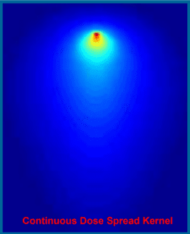
- A Kernel represents energy the energy spread resulting from an interaction at a given point or line
- The energy spreads because charged particles and scatter photons carry energy away the site of primary interaction
- Kernels are pre-calculated using complex Monte Carlo simulations
- Both line and point kernel are radially symmetric
What is Ray Tracing?
Ray tracing algorithms are used in kernel based dose calculation algorithms to transport energy from the radiation source through the patient/phantom data set.
- Steps in ray tracing
- A ray is generated originating at the radiation source, projecting through the aperture (collimators, MLC, blocks, etc), and into the patient data set.
- The points of intersection between a ray and the boundary of a voxel are identified.
- These points of intersection are circled in blue in the image at right.
- For each voxel, the distance between the two points of intersection between the ray and the voxel is computed.
- Distance determined in step 3 is used to scale the fluence though the voxel as a result of the ray.
- E.g. Since the distance A-B is greater than distance C-D, voxel 2 have more fluence resulting from this ray than voxel 6.
- Proper ray sampling is important to balance calculation accuracy against computation time.
- In the example at right with only two rays voxels 8 and 11 would be assumed to have no fluence!

Kernel Based Algorithms: Pencil Beam
Pencil beam dose computation is the simplest and fastest kernel based dose computation method. Pencil beam dose calculations typically use a line kernel to model dose deposition and often neglect modifying dose deposition based on medium density. This makes pencil beam algorithms poor choice for very heterogeneous treatment sites such as the lungs.
Steps in computing pencil beam dose
- The aperture is projected through the patient/phantom and is subdivided into small beamlets.
- Pencil kernels are applied to each beamlet giving a beamlet specific dose distribution.
- These dose distributions are then simply summed resulting in the total dose map.
Kernel Based Algorithms: Convolution / Superposition Algorithms
Convolution/superposition algorithms use one or more point Kernels rather than a line Kernel. This allows the kernel to be scaled according to local and surrounding density. Additionally, multiple point kernels are typically available representing dose deposition of different energy ranges in the clinical beam. This allows the algorithm to accurately model beam hardening as the beam traverses the medium. Advanced algorithms will include a kernel tilting component which shifts the orientation of the kernel to match the diverging primary beam.
To compute dose, the Kernal is convolved with TERMA (Total Energy Released per unit MAss) yielding absorbed dose. Convolution, ⊗, is a mathematical operation used to combine functions.
![]()
Steps in computing convolution/superposition dose
- Model primary photons incident on the phantom/patient.
- A finite source size and location is determined in commissioning.
- Mask function is a mathematical expression defining the outlines of collimators and MLC/block position.
- The mask function reduces transmission of in the blocked areas by a factor determined in commissioning.
- Aperture function is used to model the penumbra blurring the results from collimator and MLC positions.
- Aperture functions shape is that of a normal function defined by the finite source size and location. This allows the aperture function to account for magnification effects.
- Extrafocal radiation is modeled by the addition of broad normally distributed fluence map to the fluence map produced by the primary source, mask function, and aperture function.
- Extrafocal radiation is also produced by Compton scattering in the flattening filter and, to a small degree, in other treatment head components. This causes fluence outside the mask to be higher than would be accounted for by attenuated primary photons alone.
- Ray-tracing projects fluence through the phantom/patient.
- TERMA is calculated from fluence and mass attenuation coefficient.

- Ray attenuation is based on voxel density and the energy fluence spectrum.
- Energy fluence spectrum changes as the beam hardens with depth.
- It is common to use a fluence attenuation table (FAT), which maps attenuation as a function of depth and density, for this purpose.
- Dose is computed by convolution of TERMA and the Kernel.
- D = TERMA⊗K
- Kernel Tilting
- The orientation of the Kernel, which is radially symmetric, should ideally align with the vector of the photon interaction with the medium.
- To accomplish this the Kernel may be tilted – its axis reoriented in space – to align with the beam’s divergence.
- Kernel tilting has only been shown to result in a minor improvement in calculation accuracy.1
- Superposition
- Phantom heterogeneities greatly influence scatter, dose, and, by extension, Kernel. For a perfect calculation, each voxel would require its own Kernel based on the density and material of itself and its surrounding voxels.
- Superposition solves this problem by scaling the Kernel according to the radiologic distance.
- Radiologic distance = (ρr – ρr’ ) · (r-r’)
- r is the location of photon interaction
- r’ is the location of dose deposition
- ρ is physical density
- Radiologic distance = (ρr – ρr’ ) · (r-r’)
- There are additionally several techniques for applying the convolution.
- Direct Summation
- Directly applies the kernel to TERMA in each dose calculation
- Very computationally expensive but allows superposition
- Scales as N6 where N is the number of voxels!
- Fast Fourier Transforms (FFT)
- Uses Fast Fourier Tranform, FFT(f ⊗ g) = FFT(f) · FFT(g), to simplify the convolution process and reduce calculation times.
- Scales as N3log(N) where N is the number of voxels.
- Cannot use superposition making FFT less accurate.
- Uses Fast Fourier Tranform, FFT(f ⊗ g) = FFT(f) · FFT(g), to simplify the convolution process and reduce calculation times.
- Collapsed Cone Convolution (CCC)
- Speeds up calculation reducing the point Kernel from a full 3D object to a point and a finite number of rays projecting away from the primary interaction site.
- Consider the Kernel to be a soccer ball with each shell composed of patches. If these patches are projected to the center of the ball, each forms a cone. CCC turns each of these cones into a single ray which may be ray traced to deposit dose.
- Speeds up calculation reducing the point Kernel from a full 3D object to a point and a finite number of rays projecting away from the primary interaction site.
- Direct Summation
- Electron contamination dose is added to dose distribution.
- For MV beams, most surface dose arises from electrons scattered in the treatment head.
- The spectrum of contaminant electrons agrees approximately with that of an electron beam with a practical range slightly greater than depth of maximum dose for the photon beam.
Boltzmann Transport Dose Computation
![]()
- The Boltzmann Transport Equation describes the behavior of radiation traveling through mater at a macroscopic level.
- Ψ is energy fluence
- σt is total interaction cross section
- Ω is particle energy fluence vector (direction)
- Q is initial energy
- May be directly solved (e.g. Eclipse Acuros) or solved by simulation (i.e. Monte Carlo)
- Assumptions
- Radiation particles interact only with medium, not with each other.
- The number of particles emitted from the source is equal to the number of particles transported plus the number absorbed.
Steps in Computing Boltzmann Transport Equation Dose
- Ray tracing transports primary fluence from source through patient/phantom.
- Calculate scattered photon fluence through patient/phantom.
- Calculate scattered electron fluence though patient/phantom.
- Compute dose.
Monte Carlo Dose Computation
Monte Carlo (MC) is a method of finding numerical solutions to a problem by random simulation. MC may be used to compute dose distributions by simulating the interactions of a large number of particles (photons, electrons, protons, etc) as they travel through a medium. Further, random noise is inherent in the MC method requiring about 104 histories (simulated particle interactions) per voxel to achieve ±1% calculation accuracy. Because MC simulates large numbers of interactions at an atomic level, it is both the most accurate and most computationally intensive method of dose calculation.
![]()
Steps in computing Monte Carlo Dose
- A particle is created by simulation traveling along a vector determined by random weighted probability.
- The distance to the particle’s next interaction is randomly assigned based on the linear attenuation coefficient of the material the particle passes through.
- Ray tracing transports the particle to the interaction site.
- The type of interaction site and determine the type of interaction taking place based on known interaction probabilities.
- Simulate the interaction which may involve energy deposit, scattering, release of additional particles to be tracked, etc.
- Steps 1-5 repeat until each the particle’s energy is below a threshold energy. At that point the remaining energy is deposited locally as dose.
- Threshold energy impacts both the speed and accuracy of calculation with higher thresholds speeding calculation at the expense of reduced accuracy.
Techniques for accelerating Monte Carlo calculations
Variance reduction
- Variance reduction techniques simplify the physics modeled in the MC simulation.
- Bremsstrahlung Splitting is a common method of variance reduction.
- Rather than randomly determining a single direction and energy for a Bremsstrahlung photon, the photon may be “split” into several photons of lower “weights” (i.e. the reduces weight photon will deliver less dose than its energy would entail but travel the same distance). This reduces the statistical noise and thereby reduces the total number of primary photons that must me simulated.
Condensed histories
- Groups and simplifies interactions that don’t appreciably change the energy or direction of the particle.
- Divides interactions into “hard” and “soft” collisions.
- Hard collisions are those which have a large impact on particle energy and direction. Hard collisions are treated normally.
- Soft collisions of those with little impact on the energy and direction. All soft collisions bounded between hard collisions are treated as a group with the hard collision. Soft collisions may also be grouped and treated at regular intervals rather than only during hard collision events.
Russian Roulette
- Rejects particles most particles unlikely to play a role in final dose.
- E.g. secondary electrons created in treatment head.
- Retains a fraction of these particles, hence the name “Russian Roulette.”
Range Rejection
- When an electron has low enough energy that it cannot reach another voxel, its energy is assumed to be deposited locally.
- This overestimates dose as it ignores potential low energy Bremsstrahlung photon production.
Phase Space Files
- A full Monte Carlo simulation would take electrons emerging from the bending magnets and model their interactions through the treatment head (target, flattening filter, scattering foil, jaws, MLC, etc) and the patient/phantom.
- To save computation time, treatment head interactions may be pre-calculated and stored in a phase space file.
- Phase space files tend to be quite large making model usage a potential bottle neck.
- This bottle neck can be avoided either by simplifying the interactions modeled in the file (i.e. use variance reduction techniques within the phase space file) or by using the phase space file to create a virtual source.
- Phase space files may also be created by physical beam measurements to create a virtual source exiting the treatment head.
Navigation
Not a Member?
Sign up today to get access to hundreds of ABR style practice questions.